
Find Edges in Shortest Paths
HardPrompt
You are given an undirected weighted graph of n nodes numbered from 0 to n - 1. The graph consists of m edges represented by a 2D array edges, where edges[i] = [ai, bi, wi] indicates that there is an edge between nodes ai and bi with weight wi.
Consider all the shortest paths from node 0 to node n - 1 in the graph. You need to find a boolean array answer where answer[i] is true if the edge edges[i] is part of at least one shortest path. Otherwise, answer[i] is false.
Return the array answer.
Note that the graph may not be connected.
Example 1:
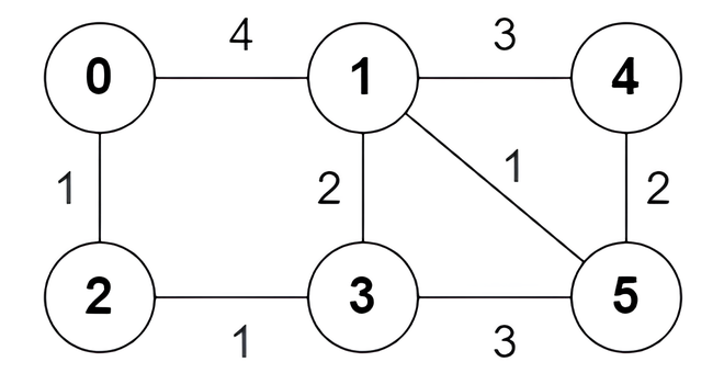
Input: n = 6, edges = [[0,1,4],[0,2,1],[1,3,2],[1,4,3],[1,5,1],[2,3,1],[3,5,3],[4,5,2]]
Output: [true,true,true,false,true,true,true,false]
Explanation:
The following are all the shortest paths between nodes 0 and 5:
- The path
0 -> 1 -> 5: The sum of weights is4 + 1 = 5. - The path
0 -> 2 -> 3 -> 5: The sum of weights is1 + 1 + 3 = 5. - The path
0 -> 2 -> 3 -> 1 -> 5: The sum of weights is1 + 1 + 2 + 1 = 5.
Example 2:
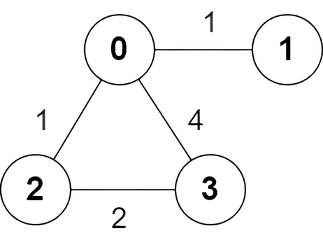
Input: n = 4, edges = [[2,0,1],[0,1,1],[0,3,4],[3,2,2]]
Output: [true,false,false,true]
Explanation:
There is one shortest path between nodes 0 and 3, which is the path 0 -> 2 -> 3 with the sum of weights 1 + 2 = 3.
Constraints:
2 <= n <= 5 * 104m == edges.length1 <= m <= min(5 * 104, n * (n - 1) / 2)0 <= ai, bi < nai != bi1 <= wi <= 105- There are no repeated edges.
Approaches
3 approaches with complexity analysis and trade-offs.
This approach involves finding all possible simple paths from node 0 to node n-1. For each path, we calculate its total weight. We identify the minimum weight among all these paths, which is the shortest path distance. Finally, we iterate through all the edges and check if an edge is part of any path whose total weight equals the shortest path distance.
Algorithm
- Use a recursive Depth First Search (DFS) to find all simple paths from node 0 to node
n-1. - Store each path and its calculated total weight.
- After finding all paths, determine the minimum weight,
shortest_dist, among them. - Initialize a boolean array
answerof sizemto allfalse. - Iterate through each edge
edges[i]. For this edge, iterate through all the found paths. - If a path's weight is equal to
shortest_distand it containsedges[i], setanswer[i]totrueand move to the next edge.
Walkthrough
The most straightforward, yet impractical, way to solve this problem is to enumerate every possible path from the start node (0) to the end node (n-1). This can be achieved using a backtracking algorithm, typically a variation of Depth First Search (DFS), that explores all routes without visiting the same node twice within a single path.
As each path is discovered, its total weight is computed by summing the weights of its constituent edges. These paths and their weights are stored. After the search is complete, we find the minimum weight among all paths, which represents the length of the shortest path.
With the shortest path length known, we can then determine which edges belong to a shortest path. We iterate through our original list of edges. For each edge, we check if it is included in any of the paths we found that have a total weight equal to the minimum shortest path length. If it is, we mark its corresponding entry in the final answer array as true.
Complexity
Time
O(P * N), where P is the number of simple paths. The number of paths can be exponential or even factorial in the number of nodes, making this approach infeasible for anything but very small graphs.
Space
O(P * N), where P is the number of simple paths and N is the number of nodes. In the worst case, P can be as large as O(N!), making the space complexity enormous.
Trade-offs
Pros
Conceptually simple and easy to understand.
Cons
Extremely inefficient and will time out on the given constraints.
The number of simple paths in a graph can be exponential, leading to prohibitive time and memory usage.
This approach improves upon brute force by using the properties of shortest paths. First, we calculate the global shortest path distance from node 0 to n-1. Then, for each edge (u, v) with weight w, we check if it can be part of a shortest path. The condition for this is that the shortest path from 0 to u, plus the edge weight w, plus the shortest path from v to n-1, must equal the global shortest path distance. This check is performed for every single edge.
Algorithm
- Build an adjacency list representation of the graph.
- Run Dijkstra's algorithm from source 0 to compute
dist(0, x)for all nodesx. Store these in an arraydist0. - The overall shortest path length is
shortest_path_len = dist0[n-1]. - If
n-1is unreachable, all answers arefalse. - Initialize a boolean array
answerof sizemtofalse. - Iterate through each edge
edges[i] = (u, v, w):- To check the condition
dist(0, u) + w + dist(v, n-1) == shortest_path_len, we needdist(v, n-1). - Run a full Dijkstra's algorithm starting from node
vto finddist(v, n-1). - If the condition holds, set
answer[i] = true. - Also check the other direction:
dist(0, v) + w + dist(u, n-1) == shortest_path_len, which requires another Dijkstra run fromu.
- To check the condition
Walkthrough
A more refined method involves using the defining property of an edge on a shortest path. An edge (u, v) with weight w lies on a shortest path from source s to target t if dist(s, u) + w + dist(v, t) = dist(s, t).
First, we perform one run of Dijkstra's algorithm starting from node 0 to find the shortest distance from 0 to all other nodes, dist(0, x). This gives us the overall shortest path length, dist(0, n-1), and the first term, dist(0, u), for our check.
Then, we iterate through each edge (u, v) in the graph. For each edge, we need to verify the condition. We already have dist(0, u). To get dist(v, n-1), we would need to run another SSSP algorithm, like Dijkstra's, starting from node v. Since we have to do this for every edge, this approach requires running Dijkstra's algorithm m+1 times in total (one initial run, and one for each of the m edges). This is computationally expensive.
Complexity
Time
O(m * (m log n)). A single Dijkstra's run is O(m log n). This is repeated for many of the `m` edges, leading to a prohibitive total time complexity.
Space
O(m + n) for the adjacency list and distance arrays.
Trade-offs
Pros
More efficient than brute-force path enumeration.
Correctly applies the mathematical properties of shortest paths.
Cons
Very high time complexity due to running Dijkstra's algorithm repeatedly.
Will result in a 'Time Limit Exceeded' error for the given problem constraints.
This is the most efficient approach. It leverages the property that an edge (u, v) with weight w is on a shortest path from a source s to a destination t if and only if dist(s, u) + w + dist(v, t) = dist(s, t). Instead of recalculating distances for each edge, we can pre-calculate all necessary distances in just two runs of Dijkstra's algorithm: one from the source and one from the destination.
Algorithm
- Build an adjacency list for the graph.
- Create two distance arrays,
dist_from_0anddist_from_n_1, of sizen, initialized to infinity. - Run Dijkstra's algorithm starting from node 0 to populate
dist_from_0. Setdist_from_0[0] = 0initially. - Run Dijkstra's algorithm starting from node
n-1to populatedist_from_n_1. Setdist_from_n_1[n-1] = 0initially. - Get the shortest path length:
shortest_path_len = dist_from_0[n-1]. - If
shortest_path_lenis infinity,n-1is unreachable. Return an array ofmfalsevalues. - Create a boolean array
answerof sizem. - Iterate through each edge
edges[i] = (u, v, w):- Check if
dist_from_0[u] + w + dist_from_n_1[v] == shortest_path_len. - Also check if
dist_from_0[v] + w + dist_from_n_1[u] == shortest_path_len. - If either condition is true, set
answer[i] = true.
- Check if
- Return the
answerarray.
Walkthrough
The optimal solution is based on the same shortest path property but avoids redundant computations. We need two pieces of information for each node x: the shortest distance from the start node 0 to x, and the shortest distance from x to the end node n-1.
We can compute all dist(0, x) values with a single run of Dijkstra's algorithm starting from node 0.
To compute all dist(x, n-1) values, we can run Dijkstra's algorithm starting from node n-1. Since the graph is undirected, the shortest distance from x to n-1 is the same as from n-1 to x. So, this second Dijkstra run gives us all the dist(n-1, x) values we need.
After these two runs, we have the overall shortest path length dist(0, n-1). If this distance is infinity, no path exists, so all edges are not on a shortest path.
Otherwise, we can iterate through every edge (u, v) with weight w just once. For each edge, we check if dist(0, u) + w + dist(n-1, v) == dist(0, n-1). Because the edge is undirected, we must also check the path through v first: dist(0, v) + w + dist(n-1, u) == dist(0, n-1). If either of these conditions is met, the edge is part of at least one shortest path, and we mark it as true in our answer array.
This approach requires only two SSSP computations, making it highly efficient.
class Solution { public boolean[] findAnswer(int n, int[][] edges) { List<List<int[]>> adj = new ArrayList<>(); for (int i = 0; i < n; i++) { adj.add(new ArrayList<>()); } for (int[] edge : edges) { adj.get(edge[0]).add(new int[]{edge[1], edge[2]}); adj.get(edge[1]).add(new int[]{edge[0], edge[2]}); } long[] distFrom0 = dijkstra(0, n, adj); long[] distFromN1 = dijkstra(n - 1, n, adj); long shortestPathLen = distFrom0[n - 1]; boolean[] answer = new boolean[edges.length]; if (shortestPathLen == Long.MAX_VALUE) { return answer; // All false if no path exists } for (int i = 0; i < edges.length; i++) { int u = edges[i][0]; int v = edges[i][1]; int w = edges[i][2]; if (distFrom0[u] != Long.MAX_VALUE && distFromN1[v] != Long.MAX_VALUE && distFrom0[u] + w + distFromN1[v] == shortestPathLen) { answer[i] = true; } if (distFrom0[v] != Long.MAX_VALUE && distFromN1[u] != Long.MAX_VALUE && distFrom0[v] + w + distFromN1[u] == shortestPathLen) { answer[i] = true; } } return answer; } private long[] dijkstra(int startNode, int n, List<List<int[]>> adj) { long[] dist = new long[n]; Arrays.fill(dist, Long.MAX_VALUE); dist[startNode] = 0; // PriorityQueue stores {distance, node} PriorityQueue<long[]> pq = new PriorityQueue<>((a, b) -> Long.compare(a[0], b[0])); pq.offer(new long[]{0, startNode}); while (!pq.isEmpty()) { long[] current = pq.poll(); long d = current[0]; int u = (int) current[1]; if (d > dist[u]) { continue; } for (int[] edge : adj.get(u)) { int v = edge[0]; int weight = edge[1]; if (dist[u] + weight < dist[v]) { dist[v] = dist[u] + weight; pq.offer(new long[]{dist[v], v}); } } } return dist; }}Complexity
Time
O(m log n). Building the graph is O(m+n). Each of the two Dijkstra runs takes O((m+n) log n), which simplifies to O(m log n) as `m` is typically at least `n-1`. The final loop over edges is O(m). The bottleneck is the two Dijkstra calls.
Space
O(m + n). This is for the adjacency list (O(m+n)), two distance arrays (O(n)), and the priority queue used in Dijkstra's algorithm (O(n)).
Trade-offs
Pros
Optimal time complexity for this problem.
Efficiently computes all necessary distances with just two SSSP runs.
Scales well for large graphs within the given constraints.
Cons
Slightly more complex to implement than a single Dijkstra run.
Requires careful handling of large path weights to avoid integer overflow, by using 64-bit integers (long) for distances.
Solutions
Solution
class Solution {public boolean[] findAnswer(int n, int[][] edges) { List<int[]>[] g = new List[n]; Arrays.setAll(g, k->new ArrayList<>()); int m = edges.length; for (int i = 0; i < m; ++i) { int a = edges[i][0], b = edges[i][1], w = edges[i][2]; g[a].add(new int[]{b, w, i}); g[b].add(new int[]{a, w, i}); } int[] dist = new int[n]; final int inf = 1 << 30; Arrays.fill(dist, inf); dist[0] = 0; PriorityQueue<int[]> pq = new PriorityQueue<>((a, b)->a[0] - b[0]); pq.offer(new int[]{0, 0}); while (!pq.isEmpty()) { var p = pq.poll(); int da = p[0], a = p[1]; if (da > dist[a]) { continue; } for (var e : g[a]) { int b = e[0], w = e[1]; if (dist[b] > dist[a] + w) { dist[b] = dist[a] + w; pq.offer(new int[]{dist[b], b}); } } } boolean[] ans = new boolean[m]; if (dist[n - 1] == inf) { return ans; } Deque<Integer> q = new ArrayDeque<>(); q.offer(n - 1); while (!q.isEmpty()) { int a = q.poll(); for (var e : g[a]) { int b = e[0], w = e[1], i = e[2]; if (dist[a] == dist[b] + w) { ans[i] = true; q.offer(b); } } } return ans; }}class Solution { public: vector < bool > findAnswer ( int n , vector < vector < int >>& edges ) { vector < vector < array < int , 3 >>> g ( n ); int m = edges . size (); for ( int i = 0 ; i < m ; ++ i ) { auto e = edges [ i ]; int a = e [ 0 ], b = e [ 1 ], w = e [ 2 ]; g [ a ]. push_back ({ b , w , i }); g [ b ]. push_back ({ a , w , i }); } const int inf = 1 << 30 ; vector < int > dist ( n , inf ); dist [ 0 ] = 0 ; using pii = pair < int , int > ; priority_queue < pii , vector < pii > , greater < pii >> pq ; pq . push ({ 0 , 0 }); while ( ! pq . empty ()) { auto [ da , a ] = pq . top (); pq . pop (); if ( da > dist [ a ]) { continue ; } for ( auto [ b , w , _ ] : g [ a ]) { if ( dist [ b ] > dist [ a ] + w ) { dist [ b ] = dist [ a ] + w ; pq . push ({ dist [ b ], b }); } } } vector < bool > ans ( m ); if ( dist [ n - 1 ] == inf ) { return ans ; } queue < int > q { { n - 1 } }; while ( ! q . empty ()) { int a = q . front (); q . pop (); for ( auto [ b , w , i ] : g [ a ]) { if ( dist [ a ] == dist [ b ] + w ) { ans [ i ] = true ; q . push ( b ); } } } return ans ; } };class Solution: def findAnswer(self, n: int, edges: List[List[int]]) -> List[bool]: g = defaultdict(list) for i, (a, b, w) in enumerate(edges): g[a]. append((b, w, i)) g[b]. append((a, w, i)) dist = [inf] * n dist[0] = 0 q = [(0, 0)] while q: da, a = heappop(q) if da > dist[a]: continue for b, w, _ in g[a]: if dist[b] > dist[a] + w: dist[b] = dist[a] + w heappush(q, (dist[b], b)) m = len(edges) ans = [False] * m if dist[n - 1] == inf: return ans q = deque([n - 1]) while q: a = q . popleft() for b, w, i in g[a]: if dist[a] == dist[b] + w: ans[i] = True q . append(b) return ansVideo walkthrough
Newsletter
One sharp idea, every week
System design and interview prep — short enough to finish.
No spam. Unsubscribe anytime.
Practice
Same difficulty — related problems to reinforce the pattern.