
Maximize the Number of Target Nodes After Connecting Trees II
HardPrompt
There exist two undirected trees with n and m nodes, labeled from [0, n - 1] and [0, m - 1], respectively.
You are given two 2D integer arrays edges1 and edges2 of lengths n - 1 and m - 1, respectively, where edges1[i] = [ai, bi] indicates that there is an edge between nodes ai and bi in the first tree and edges2[i] = [ui, vi] indicates that there is an edge between nodes ui and vi in the second tree.
Node u is target to node v if the number of edges on the path from u to v is even. Note that a node is always target to itself.
Return an array of n integers answer, where answer[i] is the maximum possible number of nodes that are target to node i of the first tree if you had to connect one node from the first tree to another node in the second tree.
Note that queries are independent from each other. That is, for every query you will remove the added edge before proceeding to the next query.
Example 1:
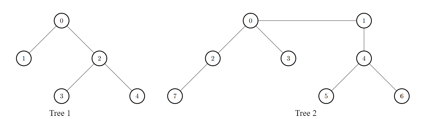
Input: edges1 = [[0,1],[0,2],[2,3],[2,4]], edges2 = [[0,1],[0,2],[0,3],[2,7],[1,4],[4,5],[4,6]]
Output: [8,7,7,8,8]
Explanation:
- For
i = 0, connect node 0 from the first tree to node 0 from the second tree. - For
i = 1, connect node 1 from the first tree to node 4 from the second tree. - For
i = 2, connect node 2 from the first tree to node 7 from the second tree. - For
i = 3, connect node 3 from the first tree to node 0 from the second tree. - For
i = 4, connect node 4 from the first tree to node 4 from the second tree.
Example 2:
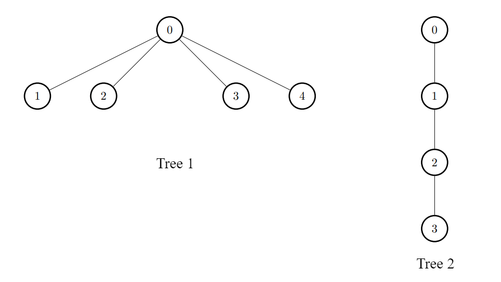
Input: edges1 = [[0,1],[0,2],[0,3],[0,4]], edges2 = [[0,1],[1,2],[2,3]]
Output: [3,6,6,6,6]
Explanation:
For every i, connect node i of the first tree with any node of the second tree.
Constraints:
2 <= n, m <= 105edges1.length == n - 1edges2.length == m - 1edges1[i].length == edges2[i].length == 2edges1[i] = [ai, bi]0 <= ai, bi < nedges2[i] = [ui, vi]0 <= ui, vi < m- The input is generated such that
edges1andedges2represent valid trees.
Approaches
3 approaches with complexity analysis and trade-offs.
This approach directly simulates the process described in the problem. For each query node i in the first tree, we exhaustively check every possible pair of nodes (u, v) (one from each tree) to form a connection. For each such connection, we calculate the total number of nodes that become target to i by finding path lengths in the newly formed combined tree. We keep track of the maximum number of targets found across all possible connections for each i.
Algorithm
- For each query node
iin the first tree (from0ton-1):- Initialize a variable
max_targets_for_ito 0. - Iterate through every possible node
uin the first tree to connect from. - Iterate through every possible node
vin the second tree to connect to.- For this specific connection
(u, v), calculate the total number of target nodes with respect toi.- To do this, we need distances. The distance between two nodes in the same tree is their path length. The distance between a node in Tree1 and a node in Tree2 is
dist1(i, u) + 1 + dist2(v, k). - We can run a Breadth-First Search (BFS) from
iin Tree1 to finddist1(i, j)for allj. - We can run a BFS from
vin Tree2 to finddist2(v, k)for allk. - Sum up the nodes
jin Tree1 wheredist1(i, j)is even and nodeskin Tree2 wheredist1(i, u) + 1 + dist2(v, k)is even.
- To do this, we need distances. The distance between two nodes in the same tree is their path length. The distance between a node in Tree1 and a node in Tree2 is
- Update
max_targets_for_iwith the maximum count found so far.
- For this specific connection
- Store the result in
answer[i].
- Initialize a variable
Walkthrough
The algorithm iterates through all n choices for the query node i. For each i, it then iterates through all n choices for the connection node u in Tree1 and all m choices for the connection node v in Tree2. Inside the innermost loop, it calculates the number of target nodes. This involves computing distances from i in Tree1 (via one BFS) and from v in Tree2 (via another BFS). This process is repeated for every single combination, leading to a very high time complexity.
// This is a conceptual representation of the brute-force logic.// A literal implementation would be too complex and inefficient to be practical.class Solution { // Helper to run BFS and get distances from a start node in a given tree private int[] bfs(int startNode, int numNodes, List<List<Integer>> adj) { int[] dist = new int[numNodes]; Arrays.fill(dist, -1); Queue<Integer> q = new LinkedList<>(); dist[startNode] = 0; q.offer(startNode); while (!q.isEmpty()) { int u = q.poll(); for (int v : adj.get(u)) { if (dist[v] == -1) { dist[v] = dist[u] + 1; q.offer(v); } } } return dist; } public int[] maximizeTargetNodes(int n, int[][] edges1, int m, int[][] edges2) { List<List<Integer>> adj1 = new ArrayList<>(); for (int i = 0; i < n; i++) adj1.add(new ArrayList<>()); for (int[] edge : edges1) { adj1.get(edge[0]).add(edge[1]); adj1.get(edge[1]).add(edge[0]); } List<List<Integer>> adj2 = new ArrayList<>(); for (int i = 0; i < m; i++) adj2.add(new ArrayList<>()); for (int[] edge : edges2) { adj2.get(edge[0]).add(edge[1]); adj2.get(edge[1]).add(edge[0]); } int[] answer = new int[n]; for (int i = 0; i < n; i++) { long maxTargets = 0; int[] distsFromI = bfs(i, n, adj1); for (int u = 0; u < n; u++) { for (int v = 0; v < m; v++) { long currentTargets = 0; // Targets in Tree1 for (int j = 0; j < n; j++) { if (distsFromI[j] % 2 == 0) { currentTargets++; } } // Targets in Tree2 int[] distsFromV = bfs(v, m, adj2); int dist_i_u = distsFromI[u]; for (int k = 0; k < m; k++) { if ((dist_i_u + 1 + distsFromV[k]) % 2 == 0) { currentTargets++; } } maxTargets = Math.max(maxTargets, currentTargets); } } answer[i] = (int) maxTargets; } return answer; }}Complexity
Time
O(n * n * m * (n + m)). For each of the `n` queries, we loop `n*m` times. Inside, we run two BFS traversals taking O(n) and O(m). This is prohibitively slow.
Space
O(n + m) to store adjacency lists and data for BFS.
Trade-offs
Pros
Simple to understand as it directly follows the problem statement.
Cons
Extremely inefficient and will time out for the given constraints.
Performs a large amount of redundant computation.
This approach improves upon the naive brute-force by avoiding redundant calculations. We observe that the optimal choice of connection (u, v) allows us to gain a fixed maximum number of targets from Tree2, regardless of the query node i. We can pre-calculate this value. Then, for each query i, we only need to determine the number of its targets within Tree1, which can be found by a single graph traversal from i.
Algorithm
- Pre-computation for Tree2:
- Realize that the maximum number of target nodes from Tree2 is independent of the query node
i. - Perform a single BFS/DFS on Tree2 to find its bipartite partitions. Count the number of nodes in each partition,
count2_evenandcount2_odd. - The maximum contribution from Tree2 will always be
max(count2_even, count2_odd).
- Realize that the maximum number of target nodes from Tree2 is independent of the query node
- Calculation for each query
i:- For each node
ifrom0ton-1:- Run a BFS/DFS on Tree1 starting from
ito find the distance to all other nodesj. - Count the number of nodes
jwheredist1(i, j)is even. This gives the number of targets within Tree1. - The total maximum targets for
iis the sum of targets from Tree1 and the pre-calculated maximum from Tree2.
- Run a BFS/DFS on Tree1 starting from
- Store this sum in
answer[i].
- For each node
Walkthrough
The core optimization is decoupling the problem. The total number of targets is targets_in_T1 + targets_in_T2. We want to maximize this sum. The choice of connection (u, v) affects targets_in_T2. A careful analysis shows that max_{u,v}(targets_in_T2) is a constant value for any i. We can pre-calculate this constant by finding the sizes of the two partitions of Tree2's bipartite coloring. Then, the problem reduces to, for each i, finding targets_in_T1. This is done by running a BFS from each i.
class Solution { // Helper to run BFS and get distances private int[] bfs(int startNode, int numNodes, List<List<Integer>> adj) { int[] dist = new int[numNodes]; Arrays.fill(dist, -1); Queue<Integer> q = new LinkedList<>(); dist[startNode] = 0; q.offer(startNode); while (!q.isEmpty()) { int u = q.poll(); for (int v : adj.get(u)) { if (dist[v] == -1) { dist[v] = dist[u] + 1; q.offer(v); } } } return dist; } public int[] maximizeTargetNodes(int n, int[][] edges1, int m, int[][] edges2) { List<List<Integer>> adj1 = new ArrayList<>(); for (int i = 0; i < n; i++) adj1.add(new ArrayList<>()); for (int[] edge : edges1) { adj1.get(edge[0]).add(edge[1]); adj1.get(edge[1]).add(edge[0]); } List<List<Integer>> adj2 = new ArrayList<>(); for (int i = 0; i < m; i++) adj2.add(new ArrayList<>()); for (int[] edge : edges2) { adj2.get(edge[0]).add(edge[1]); adj2.get(edge[1]).add(edge[0]); } // Pre-calculate max contribution from Tree2 long[] counts2 = new long[2]; int[] colors2 = new int[m]; Arrays.fill(colors2, -1); Queue<Integer> q2 = new LinkedList<>(); q2.offer(0); colors2[0] = 0; while(!q2.isEmpty()) { int u = q2.poll(); counts2[colors2[u]]++; for(int v : adj2.get(u)) { if(colors2[v] == -1) { colors2[v] = 1 - colors2[u]; q2.offer(v); } } } long maxContribT2 = Math.max(counts2[0], counts2[1]); int[] answer = new int[n]; for (int i = 0; i < n; i++) { int[] distsFromI = bfs(i, n, adj1); long targetsInT1 = 0; for (int dist : distsFromI) { if (dist % 2 == 0) { targetsInT1++; } } answer[i] = (int) (targetsInT1 + maxContribT2); } return answer; }}Complexity
Time
O(n^2 + m). We perform one O(m) traversal for Tree2. Then, for each of the `n` nodes in Tree1, we perform an O(n) traversal. This leads to O(n*n) work for Tree1.
Space
O(n + m) for adjacency lists and BFS data structures.
Trade-offs
Pros
Much faster than the naive brute-force approach.
Correctly identifies that the contribution from Tree2 can be calculated independently.
Cons
The time complexity is dominated by the O(n^2) part, which is too slow for the given constraints on
n.
This optimal approach fully leverages the properties of trees as bipartite graphs. Instead of re-calculating distances for each query, we can pre-calculate the bipartite partitions for both trees in linear time. The number of targets for any node i within its own tree is simply the size of the partition it belongs to. The maximum possible number of targets from the second tree is also a constant value determined by the sizes of its partitions. Combining these pre-calculated values gives the answer for each query in constant time.
Algorithm
- Bipartite Coloring: A node
uis target tovif the distance between them is even. In a bipartite graph (like a tree), this is equivalent touandvbeing in the same color partition. - Algorithm Steps:
- Build adjacency lists for both trees.
- Perform a single BFS/DFS on Tree1, starting from an arbitrary root (e.g., node 0), to establish a bipartite coloring. Store the color of each node in an array
color1. Also, count the number of nodes in each partition:count1_color0andcount1_color1. - Perform a single BFS/DFS on Tree2 to find the sizes of its two partitions:
count2_color0andcount2_color1. - The maximum number of target nodes from Tree2 is
max_contrib_T2 = max(count2_color0, count2_color1). - For each node
ifrom0ton-1:- The number of targets for
iwithin Tree1 are all the nodes that have the same color asi. This is eithercount1_color0orcount1_color1, which can be determined in O(1) using the pre-calculatedcolor1[i]. answer[i] = (targets in Tree1) + max_contrib_T2.
- The number of targets for
Walkthrough
The key insight is that dist(a, b) % 2 == (dist(root, a) % 2 + dist(root, b) % 2) % 2. This means two nodes are at an even distance if and only if they have the same color in a 2-coloring of the graph.
For any query i, the number of targets within Tree1 is the size of the partition i is in. We can find this by doing one traversal of Tree1 to color all nodes and count partition sizes.
For Tree2, we want to maximize |{k | (dist1(i, u) + 1 + dist2(v, k)) % 2 == 0}|. By choosing u appropriately (e.g., u=i or a neighbor of i), we can make dist1(i, u) either even or odd. This allows us to choose whether we need dist2(v, k) to be odd or even. To maximize the count, we will always choose the one that gives more nodes, which is max(count2_even, count2_odd). This value is constant for all i.
This reduces the entire problem to two initial traversals and then a simple loop, achieving linear time complexity.
class Solution { public int[] maximizeTargetNodes(int n, int[][] edges1, int m, int[][] edges2) { // Build adjacency lists List<List<Integer>> adj1 = new ArrayList<>(); for (int i = 0; i < n; i++) adj1.add(new ArrayList<>()); for (int[] edge : edges1) { adj1.get(edge[0]).add(edge[1]); adj1.get(edge[1]).add(edge[0]); } List<List<Integer>> adj2 = new ArrayList<>(); for (int i = 0; i < m; i++) adj2.add(new ArrayList<>()); for (int[] edge : edges2) { adj2.get(edge[0]).add(edge[1]); adj2.get(edge[1]).add(edge[0]); } // Bipartite coloring for Tree 1 int[] color1 = new int[n]; Arrays.fill(color1, -1); Queue<Integer> q1 = new LinkedList<>(); q1.offer(0); color1[0] = 0; while (!q1.isEmpty()) { int u = q1.poll(); for (int v : adj1.get(u)) { if (color1[v] == -1) { color1[v] = 1 - color1[u]; q1.offer(v); } } } long count1_color0 = 0; for (int c : color1) { if (c == 0) count1_color0++; } long count1_color1 = n - count1_color0; // Bipartite coloring for Tree 2 long[] counts2 = new long[2]; int[] colors2 = new int[m]; Arrays.fill(colors2, -1); Queue<Integer> q2 = new LinkedList<>(); q2.offer(0); colors2[0] = 0; while (!q2.isEmpty()) { int u = q2.poll(); counts2[colors2[u]]++; for (int v : adj2.get(u)) { if (colors2[v] == -1) { colors2[v] = 1 - colors2[u]; q2.offer(v); } } } long maxContribT2 = Math.max(counts2[0], counts2[1]); int[] answer = new int[n]; for (int i = 0; i < n; i++) { long targetsInT1 = (color1[i] == 0) ? count1_color0 : count1_color1; answer[i] = (int) (targetsInT1 + maxContribT2); } return answer; }}Complexity
Time
O(n + m). We perform one O(n) traversal for Tree1 and one O(m) traversal for Tree2. The final loop to compute answers is O(n).
Space
O(n + m) to store adjacency lists, color arrays, and BFS queues.
Trade-offs
Pros
Optimal time and space complexity.
Solves the problem efficiently for large inputs.
Cons
The logic relies on understanding the relationship between distance parity and bipartite coloring, which may not be immediately obvious.
Solutions
Solution
public class Solution { public int[] MaxTargetNodes(int[][] edges1, int[][] edges2) { var g1 = Build(edges1); var g2 = Build(edges2); int n = g1.Length, m = g2.Length; var c1 = new int[n]; var c2 = new int[m]; var cnt1 = new int[2]; var cnt2 = new int[2]; Dfs(g2, 0, -1, c2, 0, cnt2); Dfs(g1, 0, -1, c1, 0, cnt1); int t = Math.Max(cnt2[0], cnt2[1]); var ans = new int[n]; for (int i = 0; i < n; i++) { ans[i] = t + cnt1[c1[i]]; } return ans; } private List < int > [] Build(int[][] edges) { int n = edges.Length + 1; var g = new List < int > [n]; for (int i = 0; i < n; i++) { g[i] = new List < int > (); } foreach(var e in edges) { int a = e[0], b = e[1]; g[a].Add(b); g[b].Add(a); } return g; } private void Dfs(List < int > [] g, int a, int fa, int[] c, int d, int[] cnt) { c[a] = d; cnt[d]++; foreach(var b in g[a]) { if (b != fa) { Dfs(g, b, a, c, d ^ 1, cnt); } } }}class Solution {public int[] maxTargetNodes(int[][] edges1, int[][] edges2) { var g1 = build(edges1); var g2 = build(edges2); int n = g1.length, m = g2.length; int[] c1 = new int[n]; int[] c2 = new int[m]; int[] cnt1 = new int[2]; int[] cnt2 = new int[2]; dfs(g2, 0, -1, c2, 0, cnt2); dfs(g1, 0, -1, c1, 0, cnt1); int t = Math.max(cnt2[0], cnt2[1]); int[] ans = new int[n]; for (int i = 0; i < n; ++i) { ans[i] = t + cnt1[c1[i]]; } return ans; }private List<Integer>[] build(int[][] edges) { int n = edges.length + 1; List<Integer>[] g = new List[n]; Arrays.setAll(g, i->new ArrayList<>()); for (var e : edges) { int a = e[0], b = e[1]; g[a].add(b); g[b].add(a); } return g; } private void dfs(List<Integer>[] g, int a, int fa, int[] c, int d, int[] cnt) { c[a] = d; cnt[d]++; for (int b : g[a]) { if (b != fa) { dfs(g, b, a, c, d ^ 1, cnt); } } }}class Solution {public: vector<int> maxTargetNodes(vector<vector<int>> &edges1, vector<vector<int>> &edges2) { auto g1 = build(edges1); auto g2 = build(edges2); int n = g1.size(), m = g2.size(); vector<int> c1(n, 0), c2(m, 0); vector<int> cnt1(2, 0), cnt2(2, 0); dfs(g2, 0, -1, c2, 0, cnt2); dfs(g1, 0, -1, c1, 0, cnt1); int t = max(cnt2[0], cnt2[1]); vector<int> ans(n); for (int i = 0; i < n; ++i) { ans[i] = t + cnt1[c1[i]]; } return ans; } private: vector<vector<int>> build(const vector<vector<int>> &edges) { int n = edges.size() + 1; vector<vector<int>> g(n); for (const auto &e : edges) { int a = e[0], b = e[1]; g[a].push_back(b); g[b].push_back(a); } return g; } void dfs(const vector<vector<int>> &g, int a, int fa, vector<int> &c, int d, vector<int> &cnt) { c[a] = d; cnt[d]++; for (int b : g[a]) { if (b != fa) { dfs(g, b, a, c, d ^ 1, cnt); } } }};class Solution: def maxTargetNodes(self, edges1: List[List[int]], edges2: List[List[int]]) -> List[int]: def build(edges: List[List[int]]) -> List[List[int]]: n = len(edges) + 1 g = [[] for _ in range(n)] for a, b in edges: g[a]. append(b) g[b]. append(a) return g def dfs(g: List[List[int]], a: int, fa: int, c: List[int], d: int, cnt: List[int]): c[a] = d cnt[d] += 1 for b in g[a]: if b != fa: dfs(g, b, a, c, d ^ 1, cnt) g1 = build(edges1) g2 = build(edges2) n, m = len(g1), len(g2) c1 = [0] * n c2 = [0] * m cnt1 = [0, 0] cnt2 = [0, 0] dfs(g2, 0, - 1, c2, 0, cnt2) dfs(g1, 0, - 1, c1, 0, cnt1) t = max(cnt2) return [t + cnt1[c1[i]] for i in range(n)]Video walkthrough
Newsletter
One sharp idea, every week
System design and interview prep — short enough to finish.
No spam. Unsubscribe anytime.
Practice
Same difficulty — related problems to reinforce the pattern.