
Maximum Score From Grid Operations
HardPrompt
You are given a 2D matrix grid of size n x n. Initially, all cells of the grid are colored white. In one operation, you can select any cell of indices (i, j), and color black all the cells of the jth column starting from the top row down to the ith row.
The grid score is the sum of all grid[i][j] such that cell (i, j) is white and it has a horizontally adjacent black cell.
Return the maximum score that can be achieved after some number of operations.
Example 1:
Input: grid = [[0,0,0,0,0],[0,0,3,0,0],[0,1,0,0,0],[5,0,0,3,0],[0,0,0,0,2]]
Output: 11
Explanation:
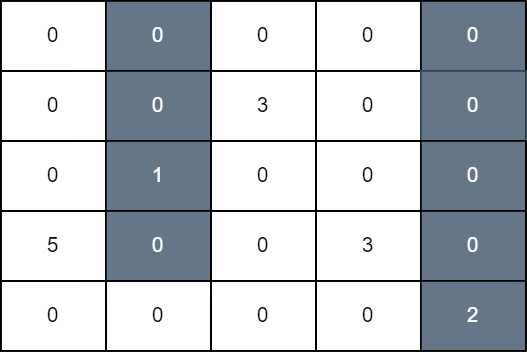
In the first operation, we color all cells in column 1 down to row 3, and in the second operation, we color all cells in column 4 down to the last row. The score of the resulting grid is grid[3][0] + grid[1][2] + grid[3][3] which is equal to 11.
Example 2:
Input: grid = [[10,9,0,0,15],[7,1,0,8,0],[5,20,0,11,0],[0,0,0,1,2],[8,12,1,10,3]]
Output: 94
Explanation:
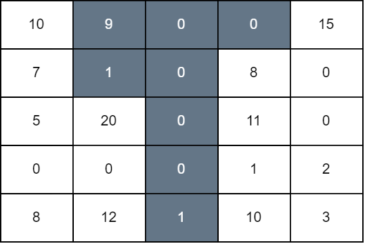
We perform operations on 1, 2, and 3 down to rows 1, 4, and 0, respectively. The score of the resulting grid is grid[0][0] + grid[1][0] + grid[2][1] + grid[4][1] + grid[1][3] + grid[2][3] + grid[3][3] + grid[4][3] + grid[0][4] which is equal to 94.
Constraints:
1 <= n == grid.length <= 100n == grid[i].length0 <= grid[i][j] <= 109
Approaches
3 approaches with complexity analysis and trade-offs.
This approach explores every possible combination of operations. For each of the n columns, we can choose to color it black down to any row i (from 0 to n-1), or not color it at all. This gives n+1 choices for each column. A recursive function can be defined to try all these choices and find the one that yields the maximum score.
Algorithm
- Define a recursive function, say
solve(col, choices), wherecolis the current column index andchoicesis an array storing the chosen cutoff row for each column processed so far. - The base case for the recursion is when
col == n. At this point, a choice has been made for every column. Calculate the total score for this configuration. - To calculate the score, iterate through the grid. A cell
(r, c)is black ifr <= choices[c]. A white cell(r, c)contributes its valuegrid[r][c]to the score if it has a horizontally adjacent black cell. - In the recursive step, for the current
col, iterate through alln+1possible choices for the cutoff row (from-1ton-1, where-1signifies no operation on the column). For each choice, make a recursive callsolve(col + 1, choices). - Maintain a global variable to keep track of the maximum score found across all configurations.
Walkthrough
The core idea is to use recursion with backtracking to explore the entire search space of possible operations. We define a function that makes a decision for one column at a time.
For each column, we have n+1 options: either don't perform an operation (which we can represent with a cutoff row of -1) or perform an operation on cell (i, j) for i from 0 to n-1. This means for each column j, the number of black cells from the top can be anything from 0 to n.
Our recursive function solve(col, choices) will try each of these n+1 options for col, and then recursively call itself for the next column col + 1. When col reaches n, we have a complete configuration defined by the choices array. We then compute the score for this configuration and update our maximum score if needed.
class Solution { long maxScore = 0; int n; int[][] grid; public long maximumScore(int[][] grid) { this.n = grid.length; this.grid = grid; // choices[j] = last black row index in column j int[] choices = new int[n]; solve(0, choices); return maxScore; } private void solve(int col, int[] choices) { if (col == n) { maxScore = Math.max(maxScore, calculateScore(choices)); return; } // Try all n+1 possibilities for the current column's operation // i = -1 means no operation (0 black cells) // i = 0..n-1 means operation on (i, col) for (int i = -1; i < n; i++) { choices[col] = i; solve(col + 1, choices); } } private long calculateScore(int[] choices) { long score = 0; for (int r = 0; r < n; r++) { for (int c = 0; c < n; c++) { // Check if cell (r, c) is white if (r > choices[c]) { boolean hasBlackNeighbor = false; // Check left neighbor if (c > 0 && r <= choices[c - 1]) { hasBlackNeighbor = true; } // Check right neighbor if (!hasBlackNeighbor && c < n - 1 && r <= choices[c + 1]) { hasBlackNeighbor = true; } if (hasBlackNeighbor) { score += grid[r][c]; } } } } return score; }}Complexity
Time
O(n^2 * (n+1)^n). There are `(n+1)^n` configurations. For each, calculating the score takes `O(n^2)`. This is too slow for the given constraints.
Space
O(n) for the recursion stack depth and the `choices` array.
Trade-offs
Pros
Conceptually simple and easy to understand.
A direct translation of the problem statement into a search algorithm.
Cons
Extremely inefficient due to its exponential time complexity.
Only feasible for very small values of
n(e.g., n < 5).
This problem exhibits optimal substructure and overlapping subproblems, making it a good candidate for dynamic programming. We can build up the solution column by column. Let dp[j][i] be the maximum score considering columns 0 to j, where column j has i cells colored black from the top. The transition to compute dp[j][i] involves iterating through all possible states of the previous column j-1 and adding the score generated at the boundary.
Algorithm
- Precompute column-wise prefix sums for the grid.
prefixSum[c][r]will store the sum ofgrid[x][c]forxfrom0tor-1. This takesO(n^2)time. - Initialize a 2D DP table
dp[n][n+1].dp[j][i]will store the max score from columns0tojwithiblack cells in columnj. - Base case: For the first column
j=0, the score is 0.dp[0][i] = 0for alli. - Iterate
jfrom1ton-1(for each column). - Inside, iterate
ifrom0ton(for each possible number of black cells in columnj). - Inside this loop, iterate
kfrom0ton(for each possible number of black cells in the previous columnj-1). - Calculate the score
costgenerated between columnj-1(withkblack cells) andj(withiblack cells) using the precomputed prefix sums. - Update
dp[j][i] = max(dp[j][i], dp[j-1][k] + cost). - The final answer is the maximum value in the last column of the
dptable:max(dp[n-1][i])fori=0..n.
Walkthrough
The state dp[j][i] represents the maximum score achievable considering columns 0 through j, with the operation on column j coloring rows 0 to i-1 black. Here, j ranges from 0 to n-1, and i (the number of black cells) ranges from 0 to n.
The transition to compute dp[j][i] is based on the states of the previous column, dp[j-1]. For each possible state k (number of black cells) in column j-1, we calculate the score generated between columns j-1 and j and add it to dp[j-1][k]. We take the maximum over all possible k.
The score generated between column j-1 (with k black cells) and column j (with i black cells) is:
sum(grid[r][j-1])forrfromktoi-1, ifi > k.sum(grid[r][j])forrfromitok-1, ifk > i.0ifi == k.
To compute these sums efficiently, we first precompute prefix sums for each column.
The recurrence relation is: dp[j][i] = max_{k=0 to n} (dp[j-1][k] + cost(k, i, j-1))
class Solution { public long maximumScore(int[][] grid) { int n = grid.length; long[][] prefixSum = new long[n][n + 1]; for (int j = 0; j < n; j++) { for (int i = 0; i < n; i++) { prefixSum[j][i + 1] = prefixSum[j][i] + grid[i][j]; } } long[][] dp = new long[n][n + 1]; // Base case dp[0][i] = 0 is handled by default initialization for (int j = 1; j < n; j++) { for (int i = 0; i <= n; i++) { long maxPrevScore = Long.MIN_VALUE; for (int k = 0; k <= n; k++) { long currentCost = 0; if (i > k) { // White cells in col j-1, black in col j currentCost = prefixSum[j - 1][i] - prefixSum[j - 1][k]; } else if (k > i) { // Black cells in col j-1, white in col j currentCost = prefixSum[j][k] - prefixSum[j][i]; } maxPrevScore = Math.max(maxPrevScore, dp[j - 1][k] + currentCost); } dp[j][i] = maxPrevScore; } } long maxScore = 0; for (int i = 0; i <= n; i++) { maxScore = Math.max(maxScore, dp[n - 1][i]); } return maxScore; }}Complexity
Time
O(n^3). We have three nested loops: `j` over `n` columns, `i` over `n+1` states, and `k` over `n+1` previous states. Precomputation of prefix sums takes `O(n^2)`.
Space
O(n^2) for the `dp` table and `O(n^2)` for prefix sums. The DP table space can be optimized to `O(n)` by only storing the previous column's results, but the total remains `O(n^2)`.
Trade-offs
Pros
Significantly more efficient than brute force.
Guaranteed to find the optimal solution.
The logic is a standard DP formulation for path/sequence problems.
Cons
The
O(n^3)complexity might be too slow and could lead to a 'Time Limit Exceeded' error forn=100.
The O(N^3) DP approach can be optimized by observing that the inner loop over k is essentially finding a maximum value. By rearranging the terms in the recurrence relation, we can separate the parts dependent on k from those dependent on i. This allows us to precompute the required maximums for all i in a single pass, reducing the complexity of processing each column from O(n^2) to O(n).
Algorithm
- Precompute column-wise prefix sums
prefixSum[c][r]inO(n^2). - Initialize
dp_prevarray of sizen+1with zeros (for column 0). - Iterate
jfrom1ton-1. - Inside the loop, compute two temporary arrays based on
dp_prevand prefix sums:temp_left[k] = dp_prev[k] - prefixSum[j-1][k]andtemp_right[k] = dp_prev[k] + prefixSum[j][k]fork=0..n. - Compute a
leftMaxarray whereleftMax[i]stores the prefix maximum oftemp_left[k]fork < i. This takesO(n). - Compute a
rightMaxarray whererightMax[i]stores the suffix maximum oftemp_right[k]fork > i. This takesO(n). - Create a
dp_currarray. Iterateifrom0tonand calculatedp_curr[i]inO(1)using theleftMaxandrightMaxarrays and the optimized recurrence. - After the inner loop, update
dp_prev = dp_curr. - The final answer is the maximum value in the final
dp_prevarray.
Walkthrough
We start with the same DP state dp[j][i] as the naive DP. The key is to optimize the transition. The recurrence can be split into three cases based on the relationship between i (number of black cells in column j) and k (number of black cells in column j-1):
dp[j][i] = max(
max_{k < i} (dp[j-1][k] + prefixSum[j-1][i] - prefixSum[j-1][k]),
dp[j-1][i],
max_{k > i} (dp[j-1][k] + prefixSum[j][k] - prefixSum[j][i])
)
By factoring out terms not dependent on k from the max operations, we get:
dp[j][i] = max(
prefixSum[j-1][i] + max_{k < i} (dp[j-1][k] - prefixSum[j-1][k]),
dp[j-1][i],
-prefixSum[j][i] + max_{k > i} (dp[j-1][k] + prefixSum[j][k])
)
For a fixed j, the terms max_{k < i} (...) and max_{k > i} (...) can be precomputed for all i in O(n) time using prefix and suffix maximum arrays. This reduces the overall complexity to O(n^2).
class Solution { public long maximumScore(int[][] grid) { int n = grid.length; long[][] prefixSum = new long[n][n + 1]; for (int j = 0; j < n; j++) { for (int i = 0; i < n; i++) { prefixSum[j][i + 1] = prefixSum[j][i] + grid[i][j]; } } long[] dp = new long[n + 1]; // Represents dp_prev for the current column for (int j = 1; j < n; j++) { long[] next_dp = new long[n + 1]; long[] tempLeft = new long[n + 1]; long[] tempRight = new long[n + 1]; for (int k = 0; k <= n; k++) { tempLeft[k] = dp[k] - prefixSum[j - 1][k]; tempRight[k] = dp[k] + prefixSum[j][k]; } long[] leftMax = new long[n + 1]; leftMax[0] = Long.MIN_VALUE / 2; // Use a small enough value for (int i = 1; i <= n; i++) { leftMax[i] = Math.max(leftMax[i - 1], tempLeft[i - 1]); } long[] rightMax = new long[n + 1]; rightMax[n] = Long.MIN_VALUE / 2; for (int i = n - 1; i >= 0; i--) { rightMax[i] = Math.max(rightMax[i + 1], tempRight[i + 1]); } for (int i = 0; i <= n; i++) { long val1 = prefixSum[j - 1][i] + leftMax[i]; long val2 = dp[i]; long val3 = -prefixSum[j][i] + rightMax[i]; next_dp[i] = Math.max(val1, Math.max(val2, val3)); } dp = next_dp; } long maxScore = 0; for (long score : dp) { maxScore = Math.max(maxScore, score); } return maxScore; }}Complexity
Time
O(n^2). Precomputation of prefix sums is `O(n^2)`. The main loop runs `n-1` times for each column. Inside, computing the helper arrays and the next DP state each takes `O(n)`. Total time is `O(n^2 + n * n) = O(n^2)`.
Space
O(n^2). `O(n^2)` for prefix sums, which dominates the `O(n)` space required for the DP arrays (`dp`, `next_dp`, `leftMax`, `rightMax`).
Trade-offs
Pros
Most efficient solution with polynomial time complexity.
Passes within the time limits for the given constraints (
n <= 100).
Cons
The implementation is more complex due to the optimization and careful index management.
Video walkthrough
Newsletter
One sharp idea, every week
System design and interview prep — short enough to finish.
No spam. Unsubscribe anytime.
Practice
Same difficulty — related problems to reinforce the pattern.