Shortest Path in a Weighted Tree
HARDDescription
You are given an integer n and an undirected, weighted tree rooted at node 1 with n nodes numbered from 1 to n. This is represented by a 2D array edges of length n - 1, where edges[i] = [ui, vi, wi] indicates an undirected edge from node ui to vi with weight wi.
You are also given a 2D integer array queries of length q, where each queries[i] is either:
[1, u, v, w']– Update the weight of the edge between nodesuandvtow', where(u, v)is guaranteed to be an edge present inedges.[2, x]– Compute the shortest path distance from the root node 1 to nodex.
Return an integer array answer, where answer[i] is the shortest path distance from node 1 to x for the ith query of [2, x].
Example 1:
Input: n = 2, edges = [[1,2,7]], queries = [[2,2],[1,1,2,4],[2,2]]
Output: [7,4]
Explanation:
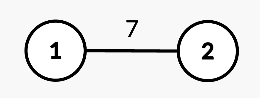
- Query
[2,2]: The shortest path from root node 1 to node 2 is 7. - Query
[1,1,2,4]: The weight of edge(1,2)changes from 7 to 4. - Query
[2,2]: The shortest path from root node 1 to node 2 is 4.
Example 2:
Input: n = 3, edges = [[1,2,2],[1,3,4]], queries = [[2,1],[2,3],[1,1,3,7],[2,2],[2,3]]
Output: [0,4,2,7]
Explanation:
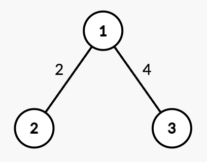
- Query
[2,1]: The shortest path from root node 1 to node 1 is 0. - Query
[2,3]: The shortest path from root node 1 to node 3 is 4. - Query
[1,1,3,7]: The weight of edge(1,3)changes from 4 to 7. - Query
[2,2]: The shortest path from root node 1 to node 2 is 2. - Query
[2,3]: The shortest path from root node 1 to node 3 is 7.
Example 3:
Input: n = 4, edges = [[1,2,2],[2,3,1],[3,4,5]], queries = [[2,4],[2,3],[1,2,3,3],[2,2],[2,3]]
Output: [8,3,2,5]
Explanation:
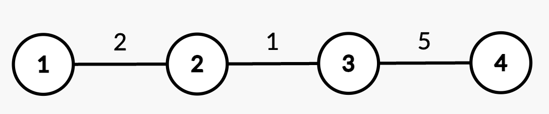
- Query
[2,4]: The shortest path from root node 1 to node 4 consists of edges(1,2),(2,3), and(3,4)with weights2 + 1 + 5 = 8. - Query
[2,3]: The shortest path from root node 1 to node 3 consists of edges(1,2)and(2,3)with weights2 + 1 = 3. - Query
[1,2,3,3]: The weight of edge(2,3)changes from 1 to 3. - Query
[2,2]: The shortest path from root node 1 to node 2 is 2. - Query
[2,3]: The shortest path from root node 1 to node 3 consists of edges(1,2)and(2,3)with updated weights2 + 3 = 5.
Constraints:
1 <= n <= 105edges.length == n - 1edges[i] == [ui, vi, wi]1 <= ui, vi <= n1 <= wi <= 104- The input is generated such that
edgesrepresents a valid tree. 1 <= queries.length == q <= 105queries[i].length == 2or4queries[i] == [1, u, v, w']or,queries[i] == [2, x]1 <= u, v, x <= n(u, v)is always an edge fromedges.1 <= w' <= 104
Approaches
Checkout 3 different approaches to solve Shortest Path in a Weighted Tree. Click on different approaches to view the approach and algorithm in detail.
Efficient Approach: Fenwick Tree on Flattened Tree
The key observation for an efficient solution is that an edge weight update affects all nodes in a specific subtree uniformly. This pattern of "range updates" (on a subtree) and "point queries" (for a node's distance) suggests using a specialized data structure. By linearizing the tree using DFS start and end times, we can map the subtree updates to range updates on an array. A Fenwick Tree (or a Segment Tree) is an excellent tool for handling these operations efficiently.
Algorithm
- Preprocessing:
- Build an adjacency list.
- Perform a DFS from the root (node 1) to compute:
initial_dist[i]: The initial distance from the root to nodei.parent[i]: The parent of nodei.startTime[i]andendTime[i]: The entry and exit times for each node in the DFS traversal. This linearizes the tree such that all nodes in a subtree ofvhave start times in the range[startTime[v], endTime[v]].
- Data Structure:
- Initialize a Fenwick Tree (BIT) of size
Nwith all zeros. This BIT will store the accumulated delta changes.
- Initialize a Fenwick Tree (BIT) of size
- Query Processing:
- For an update query
[1, u, v, w']:- Determine the child node (e.g.,
v). - Calculate
delta = w' - w_old. - This
deltaapplies to all nodes in the subtree ofv. In our linearized representation, this corresponds to the range of start times[startTime[v], endTime[v]]. - Perform a range update on the BIT:
bit.add(startTime[v], delta)andbit.add(endTime[v] + 1, -delta).
- Determine the child node (e.g.,
- For a distance query
[2, x]:- The total change in distance for node
xis the sum of all deltas for ranges that includestartTime[x]. This can be found with a point query on our BIT structure, which isbit.query(startTime[x]). - The final distance is
initial_dist[x] + bit.query(startTime[x]).
- The total change in distance for node
- For an update query
This approach combines tree algorithms with a data structure to handle the queries efficiently.
1. Preprocessing:
We start with a DFS from the root (node 1). During this traversal, we compute several properties for each node: its parent, its initial distance from the root, and its DFS start and end times. The start time is recorded when a node is first visited, and the end time is recorded after all its descendants have been visited. This mapping ensures that for any node v, all nodes u in its subtree satisfy startTime[v] <= startTime[u] <= endTime[v].
2. Fenwick Tree for Updates and Queries:
We use a Fenwick Tree (BIT) to manage the distance modifications. A standard BIT supports point updates and prefix sum queries. To handle range updates and point queries, we can use a clever trick: to add a value delta to a range [l, r], we perform two point updates on the BIT: add(l, delta) and add(r + 1, -delta). The effect of this is that when we query the prefix sum up to an index i (query(i)), we get the sum of all deltas for ranges that start at or before i. This is exactly the total change affecting the node corresponding to time i.
3. Handling Queries:
- Update
[1, u, v, w']: We find the child node (sayv), calculatedelta, and update the BIT atstartTime[v]andendTime[v] + 1. This takesO(log N)time. - Query
[2, x]: The current distance is the initial distance plus all accumulated changes. We retrieve this by querying the BIT atstartTime[x]. The result isinitial_dist[x] + bit.query(startTime[x]). This also takesO(log N)time.
import java.util.*;

class Solution {
    private int timer;
    private int[] parent, startTime, endTime;
    private long[] initialDist;
    private List<Map<Integer, Integer>> adj;

    public long[] shortestPath(int n, int[][] edges, int[][] queries) {
        adj = new ArrayList<>();
        for (int i = 0; i <= n; i++) adj.add(new HashMap<>());
        for (int[] edge : edges) {
            adj.get(edge[0]).put(edge[1], edge[2]);
            adj.get(edge[1]).put(edge[0], edge[2]);
        }

        parent = new int[n + 1];
        startTime = new int[n + 1];
        endTime = new int[n + 1];
        initialDist = new long[n + 1];
        timer = 0;
        dfs(1, 0, 0);

        FenwickTree bit = new FenwickTree(n);
        List<Long> answers = new ArrayList<>();

        for (int[] query : queries) {
            if (query[0] == 1) {
                int u = query[1], v = query[2], w = query[3];
                if (parent[u] == v) { // Ensure u is parent of v
                    int temp = u; u = v; v = temp;
                }
                long oldWeight = adj.get(u).get(v);
                long delta = w - oldWeight;
                adj.get(u).put(v, w);
                adj.get(v).put(u, w);

                bit.add(startTime[v], delta);
                bit.add(endTime[v] + 1, -delta);
            } else {
                int x = query[1];
                long currentChange = bit.query(startTime[x]);
                answers.add(initialDist[x] + currentChange);
            }
        }

        long[] result = new long[answers.size()];
        for (int i = 0; i < answers.size(); i++) result[i] = answers.get(i);
        return result;
    }

    private void dfs(int u, int p, long currentDist) {
        parent[u] = p;
        initialDist[u] = currentDist;
        startTime[u] = ++timer;
        for (Map.Entry<Integer, Integer> entry : adj.get(u).entrySet()) {
            int v = entry.getKey();
            if (v != p) {
                dfs(v, u, currentDist + entry.getValue());
            }
        }
        endTime[u] = timer;
    }
}

class FenwickTree {
    private long[] bit;
    private int size;

    public FenwickTree(int n) {
        this.size = n;
        this.bit = new long[n + 2];
    }

    public void add(int index, long delta) {
        for (; index <= size; index += index & -index) {
            bit[index] += delta;
        }
    }

    public long query(int index) {
        long sum = 0;
        for (; index > 0; index -= index & -index) {
            sum += bit[index];
        }
        return sum;
    }
}
Complexity Analysis
Pros and Cons
- Highly efficient, with logarithmic time complexity for both updates and queries.
- Scales well for large inputs, passing the given constraints.
- It's a standard and powerful technique for a class of problems involving queries on trees.
- More complex to implement due to the need for DFS traversal times and a Fenwick Tree.
- The constant factors might be higher than simpler approaches for very small N.
Video Solution
Watch the video walkthrough for Shortest Path in a Weighted Tree
Similar Questions
5 related questions you might find useful
Algorithms:
Data Structures:
Companies:
Subscribe to Scale Engineer newsletter
Learn about System Design, Software Engineering, and interview experiences every week.
No spam, unsubscribe at any time.