
Shortest Path in Binary Matrix
MedPrompt
Given an n x n binary matrix grid, return the length of the shortest clear path in the matrix. If there is no clear path, return -1.
A clear path in a binary matrix is a path from the top-left cell (i.e., (0, 0)) to the bottom-right cell (i.e., (n - 1, n - 1)) such that:
- All the visited cells of the path are
0. - All the adjacent cells of the path are 8-directionally connected (i.e., they are different and they share an edge or a corner).
The length of a clear path is the number of visited cells of this path.
Example 1:
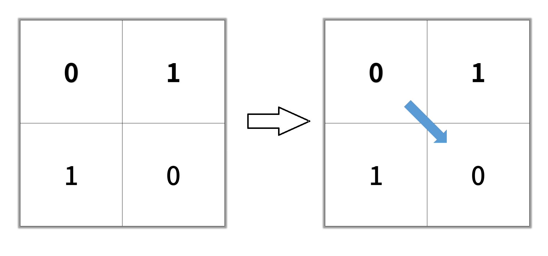
Input: grid = [[0,1],[1,0]]
Output: 2
Example 2:
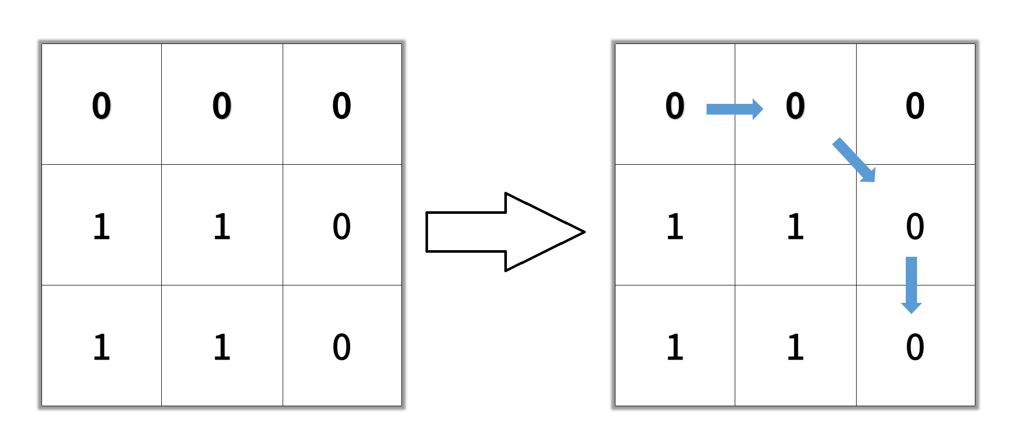
Input: grid = [[0,0,0],[1,1,0],[1,1,0]]
Output: 4
Example 3:
Input: grid = [[1,0,0],[1,1,0],[1,1,0]]
Output: -1
Constraints:
n == grid.lengthn == grid[i].length1 <= n <= 100grid[i][j] is 0 or 1
Approaches
2 approaches with complexity analysis and trade-offs.
A classic approach for finding the shortest path in an unweighted graph is the Breadth-First Search (BFS) algorithm. The binary matrix can be modeled as a graph where each cell with a value of 0 is a node, and an edge exists between any two nodes that are 8-directionally adjacent. Since each step from one cell to an adjacent one has a uniform cost (1), BFS is guaranteed to find the shortest path. It works by exploring the grid layer by layer from the starting point. The first time it reaches the destination cell, it will have done so via a path with the minimum number of steps.
Algorithm
- Check if the start
(0, 0)or end(n-1, n-1)cells are blocked (value1). If so, no path is possible, return-1. - Initialize a queue and add the starting cell
(0, 0)along with the initial path length of1. A common way to store this is a tuple or an array like{row, col, length}. - To prevent cycles and redundant computations, use a mechanism to track visited cells. A simple way is to modify the input
gridin-place, changing0s to1s as they are visited. If the input grid cannot be modified, a separateboolean[][] visitedmatrix should be used. - Mark the starting cell
(0, 0)as visited. - Start the BFS loop, which continues as long as the queue is not empty:
- Dequeue the current cell
{r, c, length}. - If the current cell is the destination
(n-1, n-1), the shortest path has been found. Return itslength. - Otherwise, explore its 8-directional neighbors:
- For each neighbor
(newR, newC):- Check if the neighbor is within the grid boundaries.
- Check if the neighbor is a clear path (value
0) and has not been visited yet. - If all checks pass, mark the neighbor as visited and enqueue it with an incremented path length:
{newR, newC, length + 1}.
- For each neighbor
- Dequeue the current cell
- If the queue becomes empty and the destination has not been reached, it means there is no clear path. Return
-1.
Walkthrough
The implementation uses a queue to manage the cells to visit. We start by adding the top-left cell (0, 0) to the queue. The algorithm then proceeds in levels. In each step, it dequeues a cell, checks if it's the destination, and if not, enqueues all its valid and unvisited neighbors. The path length is tracked along with each cell in the queue. To avoid processing a cell more than once, we mark cells as visited. A common technique is to modify the input grid itself by changing a cell's value from 0 to 1 after visiting it, which saves space by avoiding a separate visited matrix.
import java.util.LinkedList;import java.util.Queue; class Solution { public int shortestPathBinaryMatrix(int[][] grid) { int n = grid.length; if (grid[0][0] == 1 || grid[n - 1][n - 1] == 1) { return -1; } if (n == 1) { return 1; } Queue<int[]> queue = new LinkedList<>(); queue.offer(new int[]{0, 0, 1}); // {row, col, length} grid[0][0] = 1; // Mark as visited by changing the value int[][] directions = {{0, 1}, {0, -1}, {1, 0}, {-1, 0}, {1, 1}, {1, -1}, {-1, 1}, {-1, -1}}; while (!queue.isEmpty()) { int[] cell = queue.poll(); int r = cell[0]; int c = cell[1]; int length = cell[2]; for (int[] dir : directions) { int newR = r + dir[0]; int newC = c + dir[1]; if (newR >= 0 && newR < n && newC >= 0 && newC < n && grid[newR][newC] == 0) { if (newR == n - 1 && newC == n - 1) { return length + 1; } grid[newR][newC] = 1; // Mark as visited queue.offer(new int[]{newR, newC, length + 1}); } } } return -1; // Path not found }}Complexity
Time
O(N^2), where N is the side length of the grid. Each cell `(i, j)` is enqueued and dequeued at most once. For each cell, we check its 8 neighbors, which is a constant time operation.
Space
O(N^2), where N is the side length of the grid. In the worst-case scenario, the queue might need to hold a significant portion of the grid's cells. If we cannot modify the input grid, an additional O(N^2) space is required for a `visited` matrix.
Trade-offs
Pros
Guaranteed to find the shortest path in terms of the number of cells.
Relatively simple to understand and implement.
Optimal time complexity for traversing an unweighted graph, as it visits each cell at most once.
Cons
Can be memory-intensive as the queue can grow to hold a large number of cells, up to O(N^2) in the worst case.
Explores in all directions equally (like an expanding circle), which can be inefficient if the goal is in a known general direction and the grid is large.
The A* (A-star) search algorithm is an informed search algorithm that can be significantly more efficient than BFS for pathfinding problems. It improves upon BFS by using a heuristic function to prioritize which cells to explore. Instead of exploring all neighbors equally, A* favors cells that are not only close to the start (g_cost) but also seem to be closer to the destination (h_cost). This guided approach means A* often explores a much smaller portion of the grid to find the shortest path, making it faster in practice for many grid-based problems.
Algorithm
- Check if the start
(0, 0)or end(n-1, n-1)cells are blocked. If so, return-1. - Initialize a priority queue to store cells to visit. The priority will be determined by the
f_cost, which isg_cost + h_cost. g_cost: The actual distance from the start cell to the current cell (path length).h_cost: A heuristic estimate of the distance from the current cell to the end cell. For an 8-directional grid, the Chebyshev distance (max(|dx|, |dy|)) is an excellent admissible heuristic.f_cost: The estimated total cost of the path through the current cell.- Use a
dist[][]array to store the minimumg_costfound so far for each cell, initialized to infinity. This also serves as the visited set. - Add the starting cell
(0, 0)to the priority queue withg_cost = 1and its calculatedf_cost. Setdist[0][0] = 1. - While the priority queue is not empty:
- Dequeue the cell with the smallest
f_cost. Let this be{f, g, r, c}. - If
(r, c)is the destination, return itsg_cost. - If the dequeued
gis greater thandist[r][c], it means we've found a better path to this cell already, so we skip this (stale) entry. - For each of the 8 valid neighbors
(newR, newC):- Calculate the new path length to this neighbor:
new_g_cost = g + 1. - If
new_g_costis less thandist[newR][newC], it means we've found a new, shorter path to this neighbor.- Update
dist[newR][newC] = new_g_cost. - Calculate the
h_costfor the neighbor. - Enqueue the neighbor with its new costs:
{new_g_cost + h_cost, new_g_cost, newR, newC}.
- Update
- Calculate the new path length to this neighbor:
- Dequeue the cell with the smallest
- If the queue becomes empty and the destination was not reached, return
-1.
Walkthrough
A* search maintains a priority queue of cells to visit, ordered by an f_cost value. The f_cost for a cell is the sum of its g_cost (the known shortest distance from the start cell) and an h_cost (a heuristic estimate of the distance to the end cell). For this problem, with 8-directional movement, the Chebyshev distance (max(|row1 - row2|, |col1 - col2|)) is a perfect heuristic because it's admissible (it never overestimates the true cost) and consistent. The algorithm repeatedly extracts the cell with the lowest f_cost from the priority queue and explores its neighbors, updating their costs if a shorter path is found. This process continues until the destination is reached.
import java.util.Arrays;import java.util.PriorityQueue; class Solution { public int shortestPathBinaryMatrix(int[][] grid) { int n = grid.length; if (grid[0][0] == 1 || grid[n - 1][n - 1] == 1) { return -1; } // PriorityQueue stores {f_cost, g_cost, row, col} PriorityQueue<int[]> pq = new PriorityQueue<>((a, b) -> a[0] - b[0]); int[][] dist = new int[n][n]; for (int[] row : dist) { Arrays.fill(row, Integer.MAX_VALUE); } int[][] directions = {{0, 1}, {0, -1}, {1, 0}, {-1, 0}, {1, 1}, {1, -1}, {-1, 1}, {-1, -1}}; dist[0][0] = 1; // g_cost for starting cell int h_cost = Math.max(n - 1, n - 1); // Heuristic for (0,0) pq.offer(new int[]{1 + h_cost, 1, 0, 0}); while (!pq.isEmpty()) { int[] cell = pq.poll(); // int f_cost = cell[0]; int g_cost = cell[1]; int r = cell[2]; int c = cell[3]; if (r == n - 1 && c == n - 1) { return g_cost; } // If we've found a shorter path to this cell already, skip if (g_cost > dist[r][c]) { continue; } for (int[] dir : directions) { int newR = r + dir[0]; int newC = c + dir[1]; if (newR >= 0 && newR < n && newC >= 0 && newC < n && grid[newR][newC] == 0) { int new_g_cost = g_cost + 1; if (new_g_cost < dist[newR][newC]) { dist[newR][newC] = new_g_cost; int new_h_cost = Math.max(n - 1 - newR, n - 1 - newC); pq.offer(new int[]{new_g_cost + new_h_cost, new_g_cost, newR, newC}); } } } } return -1; // Path not found }}Complexity
Time
O(N^2 log N). In the worst case, A* might explore all `N^2` cells. Each operation on the priority queue (insertion and extraction) takes O(log K) time, where K is the size of the queue. Since K can be up to `N^2`, the complexity is O(N^2 log(N^2)) which simplifies to O(N^2 log N).
Space
O(N^2). The priority queue can, in the worst case, contain all `N^2` cells. The `dist` matrix also requires O(N^2) space.
Trade-offs
Pros
Generally more efficient than BFS in terms of nodes explored, especially on large grids, as it focuses the search towards the goal.
It is both complete (will find a solution if one exists) and optimal (will find the shortest path) when using an admissible heuristic.
Cons
More complex to implement compared to standard BFS due to the priority queue and heuristic calculation.
The worst-case time complexity includes a logarithmic factor, O(N^2 log N), which is theoretically slower than BFS's O(N^2). However, this is rarely a bottleneck in practice.
Solutions
Solution
class Solution {public int shortestPathBinaryMatrix(int[][] grid) { if (grid[0][0] == 1) { return -1; } int n = grid.length; grid[0][0] = 1; Deque<int[]> q = new ArrayDeque<>(); q.offer(new int[]{0, 0}); for (int ans = 1; !q.isEmpty(); ++ans) { for (int k = q.size(); k > 0; --k) { var p = q.poll(); int i = p[0], j = p[1]; if (i == n - 1 && j == n - 1) { return ans; } for (int x = i - 1; x <= i + 1; ++x) { for (int y = j - 1; y <= j + 1; ++y) { if (x >= 0 && x < n && y >= 0 && y < n && grid[x][y] == 0) { grid[x][y] = 1; q.offer(new int[]{x, y}); } } } } } return -1; }}class Solution {public: int shortestPathBinaryMatrix(vector<vector<int>> &grid) { if (grid[0][0]) { return -1; } int n = grid.size(); grid[0][0] = 1; queue<pair<int, int>> q; q.emplace(0, 0); for (int ans = 1; !q.empty(); ++ans) { for (int k = q.size(); k; --k) { auto [i, j] = q.front(); q.pop(); if (i == n - 1 && j == n - 1) { return ans; } for (int x = i - 1; x <= i + 1; ++x) { for (int y = j - 1; y <= j + 1; ++y) { if (x >= 0 && x < n && y >= 0 && y < n && !grid[x][y]) { grid[x][y] = 1; q.emplace(x, y); } } } } } return -1; }};class Solution: def shortestPathBinaryMatrix(self, grid: List[List[int]]) -> int: if grid[0][0]: return - 1 n = len(grid) grid[0][0] = 1 q = deque([(0, 0)]) ans = 1 while q: for _ in range(len(q)): i, j = q . popleft() if i == j == n - 1: return ans for x in range(i - 1, i + 2): for y in range(j - 1, j + 2): if 0 <= x < n and 0 <= y < n and grid[x][y] == 0: grid[x][y] = 1 q . append((x, y)) ans += 1 return - 1Video walkthrough
Newsletter
One sharp idea, every week
System design and interview prep — short enough to finish.
No spam. Unsubscribe anytime.
Practice
Same difficulty — related problems to reinforce the pattern.